Maximum and minimum price controls
What a price control is
- A price control is a legal limit on the price a good may be sold at.
- A control only has an effect if it binds — that is, if it stops the market reaching Pe.
- A maximum price above Pe changes nothing. A minimum price below Pe changes nothing.
- Always check which side of Pe the control sits on before you do anything else.
Maximum price control (a price ceiling)
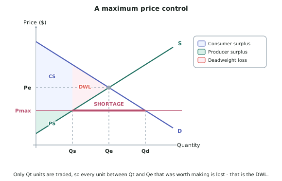
- A maximum price is a legal upper limit, set below Pe, usually to keep a good affordable.
- New Zealand's regulated electricity lines charges are an example of a price cap.
- At the controlled price:
- Quantity demanded rises to Qd, because the good is more affordable.
- Quantity supplied falls to Qs, because supplying is less profitable.
- The gap Qd − Qs is a permanent shortage — market forces cannot close it because the price is not allowed to rise.
- The quantity actually traded is Qs, the smaller of the two. You cannot buy what is not made.
Impacts
- Consumers — mixed. Those who still get the good pay less and gain surplus. Those who cannot get it at all lose everything they had. Overall CS may rise or fall.
- Producers — clearly worse off. They receive a lower price on fewer units. PS falls on both counts.
- The government — no revenue and no cost, but it must enforce the control and often ends up rationing.
- Efficiency — a deadweight loss appears between Qs and Qe. Allocatively inefficient.
- Non-price rationing appears because the price is no longer doing the job: queues, waiting lists, first-come-first-served, and black markets.
Minimum price control (a price floor)
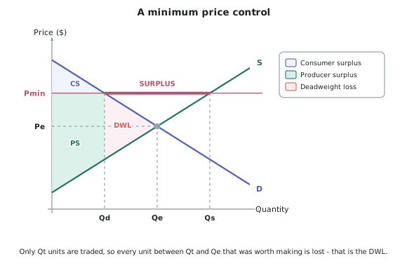
- A minimum price is a legal lower limit, set above Pe, usually to protect producers' incomes.
- The minimum wage, set by MBIE, is a minimum price in the labour market.
- At the controlled price:
- Quantity supplied rises to Qs, because supplying is more profitable.
- Quantity demanded falls to Qd, because the good is less affordable.
- The gap Qs − Qd is a permanent surplus.
- The quantity actually traded is Qd, the smaller of the two. Producers cannot force anyone to buy.
Impacts
- Consumers — clearly worse off. Higher price, fewer units. CS falls on both counts.
- Producers — mixed. Those who still sell get a higher price. Those who cannot sell lose their sales entirely. PS may rise or fall.
- The government — no revenue, and it may end up buying the surplus to support the price, which is then a cost.
- Efficiency — a deadweight loss appears between Qd and Qe. Allocatively inefficient.
The rule that makes both easy
- The short side of the market wins. Whichever of Qd and Qs is smaller is the quantity actually traded.
- Maximum price → Qs is smaller → trade at Qs.
- Minimum price → Qd is smaller → trade at Qd.
- The deadweight loss always runs from that traded quantity to Qe.
Worked ExampleA maximum price on rental housing
An illustrative rental market is in equilibrium at Pe = $600 per week and Qe = 5,000 properties.
A council imposes a maximum rent of $450 per week. At $450:
- Quantity demanded is 7,000 properties
- Quantity supplied is 3,500 properties
Identify the shortage and the quantity traded, and explain the impact on consumers, producers and allocative efficiency.
Step 1 — Check the control binds
The maximum of $450 is below the equilibrium of $600, so it does bind and the market cannot reach Pe.
Step 2 — Identify the shortage
At $450, quantity demanded (7,000) exceeds quantity supplied (3,500).
Shortage = Qd − Qs = 7,000 − 3,500 = 3,500 properties
Market forces cannot close this. The price would normally be bid up towards $600, but it is illegal to do so, so the shortage is permanent.
Step 3 — Identify the quantity traded
The short side wins. Only 3,500 properties are supplied, so only 3,500 can be rented.
Quantity traded = Qs = 3,500 properties, down from 5,000.
Step 4 — Impact on consumers
Consumers split into two groups, and both must be named:
- The 3,500 tenants who get a property pay $450 instead of $600 — a saving of $150 per week. Their individual consumer surplus rises.
- The 3,500 households in the shortage cannot rent at all. They lose all the surplus they previously had. Some of these were tenants before the control, since the market used to house 5,000.
Because 1,500 fewer properties are rented than before, and because rationing is now by queue rather than by willingness to pay, overall consumer surplus may rise or fall depending on the size of the price gain against the size of the lost quantity.
Step 5 — Impact on producers
Landlords are unambiguously worse off. They receive $450 instead of $600 on every property they still rent out, and they rent out 3,500 instead of 5,000. Producer surplus falls for both reasons — the offset between price and quantity works against them on both sides.
Step 6 — Impact on allocative efficiency
The quantity traded falls from 5,000 to 3,500, so 1,500 tenancies that used to happen no longer do. For every one of those, the demand curve lies above the supply curve — a tenant valued the property at more than it cost the landlord to provide. Those trades would have created surplus and now do not happen.
The deadweight loss is the triangle between Qs = 3,500 and Qe = 5,000, bounded by demand above and supply below. Because a deadweight loss exists, the market is allocatively inefficient.
Step 7 — The side effect the model does not draw
With 7,000 households chasing 3,500 properties and the price fixed, price can no longer ration. Something else must: waiting lists, landlords selecting tenants on other criteria, requests for payments outside the lease, or properties leaving the rental market entirely. These are predictable consequences of removing the price signal.