Topics

True, model and experimental probability

Three different things called "probability"

The explanatory notes list "true probability versus model estimates versus experimental estimates" as a method in its own right. Questions about it are almost always worth several marks, and they need words rather than arithmetic.

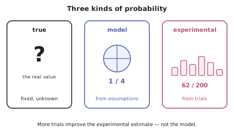
$Three panels. Left: a labelled true probability, shown as a single fixed but unknown value behind a question mark. Centre: a model estimate, shown as a fraction derived from an assumed symmetric setup. Right: an experimental estimate, shown as a relative frequency from a tally of trials, with a note that it changes each time.$

	What it is	How you get it	Does it change?
True probability	The actual long-run proportion for the real situation	You almost never know it	No — it is a fixed value
Model estimate	A probability calculated from assumptions about the situation	Arithmetic from a model	No — but it is only as good as its assumptions
Experimental estimate	The relative frequency observed in trials	Count and divide	Yes — a different set of trials gives a different value

True probability

The true probability is the proportion of times the event would occur in the long run for the real situation.
It is a fixed number and it is essentially always unknown — if you knew it, you would not need the other two.
For a real drawing pin, the true probability of landing point-up depends on its exact shape, mass distribution and the surface. No calculation can produce it.

Model estimates

A model estimate comes from assuming something about the situation and calculating.
- Assume a coin is fair → model estimate of a head is $0.5$ .
- Assume a die is fair and six-sided → model estimate of a six is $\tfrac{1}{6}$ .
- Assume births are equally likely to be boys or girls and independent → model estimate of two girls in a row is $0.25$ .
The estimate is exactly as good as the assumption. A model estimate of $0.5$ for a bent coin is a precise answer to the wrong question.
How to improve a model estimate: change the model to reflect the situation better — not by running more trials, which is what improves the other kind of estimate.

Experimental estimates

An experimental estimate is the relative frequency from actual trials:

$\text{experimental estimate} = \frac{\text{number of times the event occurred}}{\text{number of trials}}$

It varies from one set of trials to the next — this is sampling variability again, in probability clothing.
How to improve an experimental estimate: run more trials. As the number of trials increases, the relative frequency settles closer to the true probability. This is the law of large numbers, and it is why casinos are profitable and gamblers are not.

Which one does a question want?

Read for the give-aways:
- "Assuming the machine is correctly calibrated…" → model estimate
- "In 500 trials, 143 were defective…" → experimental estimate
- "The actual proportion of defective items produced by this machine" → true probability
A very common exam task: compare a model estimate with an experimental estimate and explain the difference.

Comparing a model estimate with an experimental estimate

If they differ, there are exactly two explanations, and a good answer considers both:
- Chance. Even a perfect model produces results that vary from trial to trial. A small difference in a small number of trials means nothing.
- The model is wrong. An assumption does not hold — the coin is biased, the events are not independent, the population is not what was assumed.
How to tell them apart: the size of the difference relative to the number of trials. A 3% gap in 50 trials is unremarkable; the same gap in 50 000 trials is strong evidence against the model.

Worked ExampleDistinguishing the three probabilities

A student is testing whether a spinner used in a board game is fair. The spinner has four equal-looking sectors labelled 1, 2, 3 and 4.

She spins it 200 times and records:

Sector	1	2	3	4
Frequency	41	62	48	49

(a) State the model estimate of the probability of landing on 2, and the assumption it relies on. (b) Calculate the experimental estimate of the probability of landing on 2. (c) Explain what the true probability of landing on 2 means here, and whether either estimate equals it. (d) The student concludes "the spinner is biased towards 2." Discuss.

(a) The model estimate

Step 1 — State the assumption. The four sectors are equal in size, so we assume the spinner is fair and each sector is equally likely.

Step 2 — Calculate.

$P(2) = \frac{1}{4} = 0.25$

(b) The experimental estimate

$\text{experimental estimate} = \frac{62}{200} = 0.31$

Note that this value would change if she spun another 200 times — it is an estimate produced by this particular set of trials.

(c) The true probability

(d) Evaluating the conclusion

Step 1 — Quantify the difference. The experimental estimate exceeds the model estimate by $0.31 - 0.25 = 0.06$ , or 6 percentage points. In counts, sector 2 came up 62 times when the model predicts about $200 \times 0.25 = 50$ — an excess of 12.

Step 2 — Ask whether chance could produce this. With 200 spins of a genuinely fair spinner, the count for any sector varies substantially from trial to trial. Counts anywhere in the low 40s to high 50s would be entirely unremarkable, and the other three sectors here — 41, 48, 49 — sit comfortably in that range.

An excess of 12 above the expected 50 is larger than typical but not extreme. It is the kind of result a fair spinner produces reasonably often, particularly when you consider that the student is looking at the largest of four counts — the biggest of four numbers is expected to be above average even when nothing is wrong.

Step 3 — State the conclusion properly.

The evidence is not sufficient to conclude the spinner is biased. The experimental estimate of 0.31 is higher than the model estimate of 0.25, but a difference of this size in 200 trials is consistent with chance variation in a fair spinner. The student has identified something worth checking, not something established.

What would settle it: run many more trials. Because the experimental estimate converges on the true probability as the number of trials grows (the law of large numbers), 5 000 spins would separate a genuine bias from chance. If the relative frequency for sector 2 were still near 0.31 after 5 000 spins, the model assumption of equal likelihood would be untenable and the conclusion would be justified.

A contextual point. Note also what "biased" would mean physically: the sectors would have to be unequal, or the spinner mounted off-centre. If the student can measure the sectors and finds them equal, that is independent evidence for the model and against her conclusion — and combining physical inspection with the trial data is stronger than either alone.