Topics

Probability distribution tables and graphs

What a probability distribution is

A random variable assigns a number to each outcome of a random situation — the number of cars in a queue, the number of faulty items in a box, the score on a die.
A probability distribution lists every possible value the random variable can take, together with the probability of each.
The explanatory notes name "probability distribution tables and graphs" as a method, so you must be able to build one, read one, and check one.

The table

A distribution table has the values in one row and their probabilities in the other:

$x$	0	1	2	3
$P(X = x)$	0.15	0.35	0.32	0.18

Two conditions must hold for any valid distribution:
- every probability satisfies $0 \leqslant P(X = x) \leqslant 1$
- the probabilities sum to exactly 1.
Checking the sum is the first thing to do with any distribution table, and it is how questions ask you to find a missing value.

The graph

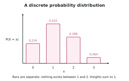
A discrete probability distribution is drawn as a bar graph with separated bars, because the variable takes only isolated values — there is nothing between 1 and 2.
The height of each bar is the probability of that value.
The heights sum to 1, which is the graphical form of the same condition.
Describe the shape in words when asked: symmetric, right-skewed (a long tail of high values), left-skewed, or uniform.

Building a distribution from a situation

The method is always the same:
- List every possible value of the random variable.
- Find the probability of each, usually with a tree, table or systematic listing.
- Check the probabilities sum to 1.
For a small situation, listing the sample space explicitly is reliable and shows the required thinking. The specification warns against guess-and-check, but systematic listing is not guess-and-check — it is a method.

Reading probabilities off a distribution

Because the values are mutually exclusive, add the relevant probabilities:
- $P(X \leqslant 2) = P(0) + P(1) + P(2)$
- $P(X \geqslant 2) = P(2) + P(3)$
- $P(X > 2) = P(3)$ — note that $>$ excludes 2 and $\geqslant$ includes it
- $P(X \neq 1) = 1 - P(1)$ , using the complement.
Inequality symbols are a genuine trap for whole-number variables. Read them twice.

Distributions of true, model and experimental probabilities

The same three-way distinction from the first page of this topic applies to whole distributions, and the explanatory notes for the companion standard make it explicit:
- a true distribution — the real long-run distribution, unknown
- a model distribution — calculated from assumptions
- an experimental distribution — the relative frequencies observed in trials.
Comparing a model distribution with an experimental one is a standard question: put them side by side, comment on where they agree and where they differ, and judge whether the differences are within what chance variation would produce.

What is not in this standard

The named distributions — binomial, Poisson and normal — and the mean and standard deviation of a random variable belong to AS91586. Here a distribution table is simply a list of values and probabilities, however it arose.

Worked ExampleBuilding and using a distribution table

A café's loyalty card gives a free drink on a customer's sixth visit. Records show that on any visit, the probability a customer buys a pastry is 0.4, independently of other visits and of other customers.

Let $X$ be the number of pastries bought by a customer across three visits.

(a) Construct the probability distribution table for $X$ . (b) Draw and describe the graph. (c) Find $P(X \geqslant 2)$ and $P(X < 2)$ . (d) Over one week the café records 200 customers who each made three visits, and observes the following counts of pastries: 0 pastries — 38 customers; 1 — 92; 2 — 58; 3 — 12. Compare this experimental distribution with the model and comment.

(a) The distribution table

Step 1 — Identify the possible values. Across three visits a customer can buy 0, 1, 2 or 3 pastries, so $X \in \{0, 1, 2, 3\}$ .

Step 2 — Find each probability using a tree. Let $p = 0.4$ be the probability of a pastry on a visit and $1 - p = 0.6$ otherwise. Visits are independent, so multiply along each path.

$P(X = 0)$ — no pastry on any of the three visits, one path:

$0.6^3 = 0.216$

$P(X = 1)$ — exactly one pastry, which can happen on the first, second or third visit — three paths, each of probability $0.4 \times 0.6 \times 0.6$ :

$3 \times 0.4 \times 0.6^2 = 3 \times 0.144 = 0.432$

$P(X = 2)$ — exactly two pastries, three paths, each $0.4^2 \times 0.6$ :

$3 \times 0.16 \times 0.6 = 3 \times 0.096 = 0.288$

$P(X = 3)$ — a pastry every visit, one path:

$0.4^3 = 0.064$

Step 3 — Assemble and check.

$x$	0	1	2	3
$P(X = x)$	0.216	0.432	0.288	0.064

$0.216 + 0.432 + 0.288 + 0.064 = 1.000 \ \checkmark$

(b) The graph and its shape

The graph is a bar chart with four separated bars at $x = 0, 1, 2, 3$ with heights 0.216, 0.432, 0.288 and 0.064.

(c) Two probabilities, watching the inequalities

$P(X \geqslant 2)$ — "at least 2" includes 2 and 3:

$P(X \geqslant 2) = 0.288 + 0.064 = 0.352$

$P(X < 2)$ — "fewer than 2" means 0 or 1, and excludes 2:

$P(X < 2) = 0.216 + 0.432 = 0.648$

Check using the complement: $1 - 0.352 = 0.648$ ✓

(d) Comparing the model with the experimental distribution

Step 1 — Convert the observed counts to relative frequencies.

$\frac{38}{200} = 0.19 \qquad \frac{92}{200} = 0.46 \qquad \frac{58}{200} = 0.29 \qquad \frac{12}{200} = 0.06$

Step 2 — Compare directly, and include the expected counts.

$x$	Model $P(X=x)$	Expected count	Observed count	Experimental
0	0.216	43.2	38	0.19
1	0.432	86.4	92	0.46
2	0.288	57.6	58	0.29
3	0.064	12.8	12	0.06

Step 3 — Comment on the agreement.

Step 4 — Judge whether the differences matter.

Step 5 — Reflect on the assumptions, since that is where a model fails first.

The model assumes visits are independent and that $p$ is the same on every visit. Both are worth questioning in context:

A customer who discovers they like the pastries may buy them more often on later visits, making visits positively dependent — which would push probability toward the extremes ( $X = 0$ and $X = 3$ ) and away from the middle.
Visits may fall on different days with different habits — a weekday morning visit and a weekend visit are not the same situation, so $p$ may not be constant.

The observed data give no sign of either problem: the extremes are not inflated. If anything, $X = 3$ came in slightly below expectation. So the model survives this comparison, and the sensible conclusion is that the assumptions are adequate for this purpose — with the caveat that 200 customers is not a large enough sample to detect a mild dependence.