Discrete random variables and their distributions
What a random variable is
- A random variable assigns a number to each outcome of a random situation.
- It is written with a capital letter (), and the values it can take with a lower-case letter (). is the probability that the variable takes the value .
- Discrete means the variable takes separate, countable values — usually whole numbers. There is nothing between 2 and 3.
- Continuous means the variable can take any value in a range, including fractions of whatever precision you like — height, time, mass.
| Situation | Variable | Type |
|---|---|---|
| Number of faulty items in a box of 50 | 0, 1, 2, …, 50 | Discrete |
| Number of texts received in an hour | 0, 1, 2, … | Discrete |
| Time until the next bus arrives | any positive number | Continuous |
| Mass of a kiwifruit | any value in a range | Continuous |
- The distinction decides which tools apply. Discrete variables have a probability for each value; continuous variables have zero probability at any exact value, and probabilities come from areas over intervals.
The distribution of a discrete random variable
- The probability distribution lists every value with its probability, as a table, a graph or a formula.
- Two conditions define a valid distribution:
- Check the sum first, every time. It is how missing values are found and how invalid tables are exposed.
The discrete uniform distribution
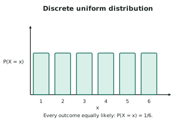
- The simplest model: outcomes, all equally likely.
- Use it when the situation has a fixed set of outcomes with no reason to favour any — a fair die, a randomly selected day of the week, a raffle ticket drawn from a drum.
- Do not use it just because a variable has several possible values. Equal likelihood is a strong assumption and usually requires a symmetric physical mechanism.
Cumulative probabilities
- The cumulative probability adds all probabilities up to and including .
- It is what your calculator's "cdf" functions give, and most exam questions need it:
| In words | How to compute |
|---|---|
| cdf at 3 | |
| cdf at 2 (whole numbers only) | |
| cdf at 2 | |
| cdf at 3 | |
| cdf at 5 cdf at 1 |
- This table is worth memorising. For a discrete variable, the difference between and is a whole bar of probability, and mixing them up is the commonest calculator error in this standard.
Building a distribution from a situation
- List every possible value.
- Find the probability of each, using a tree, a table or systematic counting.
- Check the probabilities sum to 1.
- Present it as a table, and graph it if asked.
Worked ExampleConstructing and using a distribution
A community garden has a stall where visitors draw one token at random from a bag to decide how many free seedlings they receive. The bag holds 20 tokens: 8 marked "1", 6 marked "2", 4 marked "3" and 2 marked "5".
Let be the number of seedlings a visitor receives.
(a) Write the probability distribution of as a table and check it is valid. (b) Find and . (c) Is a discrete uniform random variable? Explain. (d) The organiser wants to change the bag so that every visitor is equally likely to get 1, 2, 3 or 5 seedlings, using 20 tokens. Describe the new bag and comment on whether this is a good idea for the garden.
(a) The distribution table
Step 1 — Find each probability. Each token is equally likely, so divide the count by 20.
Step 2 — Present as a table.
| 1 | 2 | 3 | 5 | |
|---|---|---|---|---|
| 0.4 | 0.3 | 0.2 | 0.1 |
Step 3 — Check validity.
All probabilities lie between 0 and 1 ✓
Note that the value 4 does not occur — a random variable's values need not be consecutive.
(b) Two probabilities, reading the inequalities carefully
— "at least 2" includes 2, 3 and 5:
Alternatively, using the complement: ✓
— "fewer than 3" means 1 or 2, and excludes 3:
Compare with — a difference of 0.2, the whole of .
(c) Is it discrete uniform?
Step 1 — Check the definition. A discrete uniform distribution requires all outcomes to be equally likely.
Step 2 — Compare the probabilities. Here they are 0.4, 0.3, 0.2 and 0.1 — not equal.
This distinction is worth being precise about: the mechanism is uniform, the variable is not.
(d) Redesigning the bag
Step 1 — Work out the required composition. Four values, each equally likely, from 20 tokens:
Step 2 — Consider the consequence for the garden. This is the part that requires contextual thinking rather than arithmetic.
Under the original bag, the most likely outcome by far is 1 seedling (40%), and the largest prize of 5 is rare (10%). Under the new bag, the chance of 5 seedlings rises from 10% to 25%.
Step 3 — Estimate the effect on seedlings given away. Comparing the average number handed out per visitor:
Step 4 — Judge it.