Choosing and checking a distribution

The decision, in order

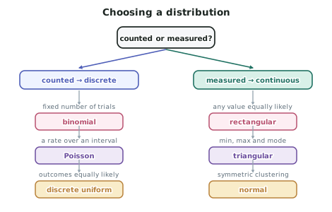
• Nearly every question in this standard begins with a choice, and the choice is made in three steps.

• Step 1 — Is the variable discrete or continuous?

  • Counting something → discrete → binomial, Poisson or discrete uniform.
  • Measuring something → continuous → rectangular, triangular or normal.

• Step 2 — For a discrete variable, is there a fixed number of trials?

  • Yes, and you could count the non-events → binomial.
  • No, only a rate over an interval → Poisson.
  • Fixed outcomes, all equally likely → discrete uniform.

• Step 3 — For a continuous variable, what shape does the context imply?

  • Every value equally likely → rectangular.
  • A minimum, maximum and most likely value → triangular.
  • Symmetric clustering around a mean → normal.

Summary of the six models

Distribution	Type	Parameters	Mean	Standard deviation
Discrete uniform	Discrete	$n$ values	average of the values	—
Binomial	Discrete	$n$, $p$	$np$	$\sqrt{np(1-p)}$
Poisson	Discrete	$\lambda$	$\lambda$	$\sqrt{\lambda}$
Rectangular	Continuous	$a$, $b$	$\frac{a+b}{2}$	$\frac{b-a}{\sqrt{12}}$
Triangular	Continuous	$a$, $b$, $c$	$\frac{a+b+c}{3}$	—
Normal	Continuous	$\mu$, $\sigma$	$\mu$	$\sigma$

True, model and experimental distributions

• The explanatory notes require you to distinguish three things, and questions ask about them directly:

	What it is	How it behaves
True distribution	The actual long-run distribution of the real situation	Fixed, and unknown
Model distribution	Calculated from a chosen model and its parameters	Fixed once chosen; only as good as its assumptions
Experimental distribution	The relative frequencies actually observed	Varies between sets of trials; converges on the true distribution as trials increase

• Improving each is different:
  • a model distribution improves by choosing a better model or better parameters
  • an experimental distribution improves by running more trials
  • the true distribution cannot be improved; it is what the other two are trying to describe.

Checking a model against data

• This is the Excellence skill in this standard. Four checks, in order of usefulness:

• 1. Compare expected counts with observed counts. Multiply each model probability by the number of trials and tabulate against what happened. This is far more informative than comparing probabilities, because it shows where the discrepancies are concentrated.

• 2. Look at the direction of the discrepancies. Scatter in both directions is chance. A systematic pattern — every low value over-predicted, every high value under-predicted — is a structural fault.

• 3. Compare the mean and the variance.

  • For a Poisson, mean should equal variance. Variance much larger means over-dispersion, so events are clustering.
  • For a binomial, the variance should be about $np(1-p)$. A larger observed variance again indicates dependence.

• 4. Check the shape. Skew in the data with a symmetric model, or a bimodal histogram with any single model, means the model is wrong regardless of its parameters.

Which assumption failed?

• When a model fits badly, name the assumption, not just the model. Almost always it is one of these:

Symptom	Likely cause
Variance much larger than the model predicts	Independence fails — a shared cause makes events cluster
Too many extreme values at both ends	The rate or probability is not constant across the data
Heavier tail on one side only	The distribution is skewed, so a symmetric model is wrong
Two peaks	Two populations mixed together
Impossible values predicted	The model is unbounded where the reality is bounded

• The recurring theme across this whole standard is that a wrong parameter is easy to fix and a wrong assumption is not. Refitting parameters to a structurally wrong model produces a model that is wrong in the same way with different numbers.