The normal distribution
What it models
- The normal distribution models measurements that cluster symmetrically around a mean, with values becoming rarer the further they are from it.
- Write it as:
- where is the mean and the standard deviation. Note the second parameter is conventionally the variance.
- Typical situations: heights and masses of people, animals or produce; measurement errors; manufactured dimensions; exam scores across a large cohort.
The shape
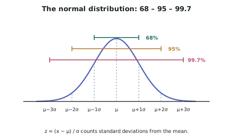
- Symmetric and bell-shaped, centred on , with .
- controls the width: a larger gives a flatter, wider curve; a smaller a taller, narrower one. The total area stays 1 either way.
- The tails extend forever in both directions but the area beyond three standard deviations is tiny.
The 68–95–99.7 rule
| Within | Approximate area |
|---|---|
| 68% | |
| 95% | |
| 99.7% |
- Use this as a sanity check on every normal calculation. If a value is 1.5 standard deviations above the mean and your calculator gives a tail probability of 0.4, something is wrong — the answer should be around 0.07.
Standardising: the -score
- The -score says how many standard deviations a value sits above (positive) or below (negative) the mean.
- Standardising converts any normal distribution to the standard normal, , which is what the booklet's tables describe.
- Even with a graphing calculator, compute the -score. It is the quantity you interpret in context — "this is 2.1 standard deviations above the mean, so it is unusual" — and it is often worth marks on its own.
Finding probabilities on a calculator
- Use normalcdf with the lower bound, upper bound, and :
| Wanted | Calculator |
|---|---|
| normalcdf | |
| normalcdf | |
| normalcdf |
- Use a very large number for an unbounded end, not the mean or zero.
- Sketch the curve and shade the region before calculating. It takes five seconds and it stops you finding the complement of what you wanted.
The inverse normal — going backwards
- When a question gives a probability and asks for the value, use invNorm.
- Typical wordings and what they need:
- "the mass exceeded by 10% of items" → invNorm with area 0.90 to the left
- "the fastest 5% of times" → for times, fastest means smallest, so area 0.05 to the left
- "the middle 90%" → two values, at areas 0.05 and 0.95.
- Most calculators take the area to the LEFT. Convert before entering, and write the conversion down.
Finding an unknown parameter
- If a question gives a probability and one of or , work backwards through the -score:
- Find from the probability using invNorm on the standard normal.
- Substitute into and solve for the unknown.
- With two unknowns you need two probability statements, giving two equations to solve simultaneously.
When a normal model is appropriate
- Use it when the data are roughly symmetric and unimodal, and the quantity results from many small independent influences added together — which is what produces a bell shape.
- Do not use it when:
- the data are clearly skewed — incomes, house prices, waiting times, rainfall
- the variable is bounded near the mean, so the tails would fall outside possible values
- the data are discrete with few values, or bimodal (often a sign of two mixed populations).
- A quick check: if is impossible — a negative time, a negative mass — the normal model fits badly at the low end and you should say so.
Worked ExampleNormal probabilities, inverse normal, and judging the model
A packhouse grades kiwifruit by mass. The masses of a variety, grams, are normally distributed with mean 95 g and standard deviation 12 g.
(a) Find the probability a randomly chosen fruit has mass over 110 g. (b) Find the probability a fruit's mass is between 85 g and 105 g. (c) The heaviest 8% are sold as premium. Find the minimum mass for premium grade. (d) Fruit lighter than 70 g is rejected. Find the expected number rejected in a bin of 400 fruit. (e) The packhouse manager says the same normal model, with the mean adjusted, will describe a new variety whose fruit are much smaller, averaging 32 g with a standard deviation of 12 g. Comment.
(a) Mass over 110 g
Step 1 — Standardise.
Step 2 — Sketch and shade the upper tail beyond .
Step 3 — Calculate.
Check against the rule: is a little above 1, and the tail beyond is about 16%, so an answer near 11% is sensible ✓
(b) Between 85 g and 105 g
Step 1 — Standardise both ends.
The two -scores are symmetric about zero, which is expected since 85 and 105 are each 10 g from the mean.
Step 2 — Calculate.
Check: the band is about , a bit narrower than (68%), so 60% is sensible ✓
(c) The premium threshold — inverse normal
Step 1 — Convert to an area on the left. The heaviest 8% lie in the upper tail, so the threshold has
Step 2 — Apply invNorm.
Step 3 — Check via the -score. on the standard normal gives , so
Interpret: premium fruit are those more than about 1.4 standard deviations above the mean mass.
(d) Expected number rejected from 400
Step 1 — Standardise.
Step 2 — Find the probability.
Step 3 — Scale to the bin.
Note the structure: this combines a normal probability with a count. Strictly the number rejected is , whose mean is — the same answer, and worth recognising as a link between the two model families.
(e) The new variety
Step 1 — Apply the check on the lower tail.
Step 2 — Quantify how bad it is.
So the model claims about 0.4% of fruit have negative mass — small, but a clear sign the model does not fit the situation.
Step 3 — Identify the real problem, which is not just the impossible values.
Step 4 — Check that fixes it.
Step 5 — Conclude.