Continuous variables and the rectangular distribution

How continuous distributions differ

• A continuous random variable can take any value in a range — a mass, a time, a length.
• Because there are infinitely many possible values, the probability of any single exact value is zero:

$$P(X = 3.5) = 0$$

• This is not a technicality to memorise and forget. It has a practical consequence:

$$P(X < a) = P(X \leqslant a)$$

• For continuous variables the inequality signs make no difference. This is the opposite of the discrete case, where they matter a great deal.

Probability is area

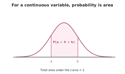
• A continuous distribution is described by a probability density function — a curve whose area gives probability.
• Two rules define any density:
  • the curve is never below zero
  • the total area under it is exactly 1.
• $P(a < X < b)$ is the area under the curve between $a$ and $b$.
• In this standard the areas come from geometry — rectangles and triangles — or from your calculator's normal functions. You are not required to integrate.

The rectangular (continuous uniform) distribution

• The rectangular distribution models a variable where every value in a range is equally likely.
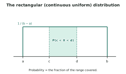
• Over the interval from $a$ to $b$, the density is a horizontal line of height:

$$\text{height} = \frac{1}{b - a}$$

• This height is exactly what makes the total area 1, since the rectangle has width $b - a$.

Finding probabilities

• For any sub-interval from $c$ to $d$ inside the range:

$$P(c < X < d) = \underbrace{(d - c)}_{\text{width}} \times \underbrace{\frac{1}{b-a}}_{\text{height}} = \frac{d - c}{b - a}$$

• In words: the probability is the fraction of the range covered. If the range is 10 minutes wide and you want a 3-minute window, the probability is 0.3.
• Trim the interval to the range first. If the variable runs from 2 to 8 and you want $P(X < 10)$, the answer is 1, not something larger.

Mean and standard deviation

$$\mu = \frac{a + b}{2} \qquad \sigma = \frac{b - a}{\sqrt{12}}$$

• The mean is the midpoint, which is obvious from the symmetry.
• The standard deviation formula is given in the booklet. As a rough check, $\sqrt{12} \approx 3.46$, so $\sigma$ is a little under a third of the range.

When a rectangular model is appropriate

• Use it when there is genuinely no reason to favour any part of the range:
  • the waiting time for a bus that runs every 15 minutes, if you arrive at a random moment
  • the position of a randomly occurring fault along a cable
  • rounding error, which is uniform across the rounding interval.
• Do not use it simply because you only know the minimum and maximum. Most real measurements cluster near a central value, and a rectangular model assumes the extremes are exactly as likely as the middle — which is usually false, and is a strong claim to make.
• The give-away in an exam question is the phrase "equally likely", "at random within", or a description with no central tendency.