Elasticity of demand
The concept
- Price elasticity of demand (PED) measures how responsive quantity demanded is to a change in price.
PED = % change in quantity demanded ÷ % change in price
- To find a percentage change: (new − old) ÷ old × 100.
- Ignore the negative sign when interpreting. The sign only reflects the law of demand.
| PED value | Name | Meaning |
|---|---|---|
| 0 | Perfectly inelastic | Quantity does not change at all |
| Between 0 and 1 | Inelastic | Quantity changes proportionately less than price |
| 1 | Unitary | Quantity changes in the same proportion |
| Above 1 | Elastic | Quantity changes proportionately more than price |
| Infinite | Perfectly elastic | Any price rise loses all sales |
What determines it
Demand is more inelastic when:
- There are few or no close substitutes — the strongest determinant by a long way.
- The good is a necessity rather than a luxury.
- It takes a small share of income.
- It is addictive or habit-forming.
- The time period is short, so consumers have not yet found alternatives.
Demand is more elastic when:
- There are many close substitutes.
- The good is a luxury.
- It takes a large share of income.
- The time period is long.
- The good is narrowly defined — one brand of milk is far more elastic than "milk", which is more elastic than "food".
Elasticity and total revenue
This is the implication a producer actually cares about, and it is where the Excellence justification usually lives.
Total revenue (TR) = price × quantity
- When the price changes, price and quantity move in opposite directions, so what happens to revenue depends on which effect is larger — which is exactly what elasticity measures.
| If demand is | And the producer raises the price | And the producer cuts the price |
|---|---|---|
| Inelastic | Quantity falls a little → revenue RISES | Quantity rises a little → revenue FALLS |
| Elastic | Quantity falls a lot → revenue FALLS | Quantity rises a lot → revenue RISES |
| Unitary | Revenue unchanged | Revenue unchanged |
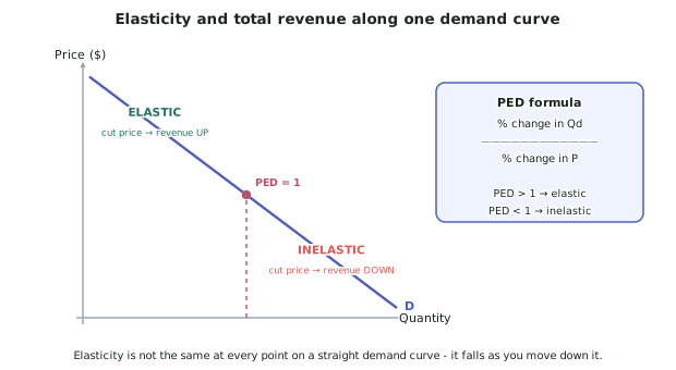
Elasticity is not the slope
- On a straight-line demand curve the slope never changes, but elasticity does: it is high at the top and low at the bottom, passing through unity at the midpoint.
- The reason is that elasticity is about percentage changes. Near the top the price is high and the quantity is small, so a given absolute change in quantity is a large percentage of a small number.
- In practice you may describe a steep curve as inelastic and a shallow one as elastic, but never write that elasticity equals the gradient.
Gathering data for this concept
- A survey: "How many would you buy at 4? At $6?" This produces a demand schedule directly.
- A class simulation: run the same market at two different prices and record the quantities.
- Real sales data from a local business before and after a price change — a rich source, and it is what an interview can obtain.
- Present it as a demand schedule table, calculate PED between the price points, and plot the demand curve.
Worked ExampleCalculating PED from survey data and advising a producer
An illustrative class survey asked 40 respondents how many bottles of a locally made sauce they would buy per month at each price.
| Price | Quantity demanded (bottles) |
|---|---|
| $4.00 | 300 |
| $5.00 | 258 |
| $6.00 | 210 |
| $7.00 | 120 |
| $8.00 | 60 |
The producer currently charges $5.00 and is considering raising the price to $6.00.
Calculate PED for that price change, interpret it, and advise the producer.
Step 1 — Calculate the percentage change in quantity demanded
Quantity falls from 258 to 210.
% change in Qd = (new − old) ÷ old × 100 % change in Qd = (210 − 258) ÷ 258 × 100 % change in Qd = −48 ÷ 258 × 100 = −18.6%
Step 2 — Calculate the percentage change in price
Price rises from $5.00 to $6.00.
% change in P = (6.00 − 5.00) ÷ 5.00 × 100 % change in P = 1.00 ÷ 5.00 × 100 = +20%
Step 3 — Calculate PED
PED = % change in Qd ÷ % change in price PED = −18.6% ÷ 20%
PED = 0.93 (ignoring the negative sign)
Step 4 — Interpret the value
0.93 is less than 1, so demand over this price range is inelastic — quantity demanded changed proportionately less than the price.
But note it is only just inelastic, sitting close to unity. That matters for the advice.
Why demand is inelastic here. The sauce is locally made and distinctive, so for buyers who want that specific product there are few very close substitutes. It also takes a small share of income, so a $1 rise is not enough to make most buyers reconsider.
Step 5 — Calculate total revenue at both prices
At $5.00: TR = $5.00 × 258 = $1,290 At $6.00: TR = $6.00 × 210 = $1,260
Revenue falls by $30.
Step 6 — Reconcile the calculation with the rule
The rule says that with inelastic demand a price rise should raise revenue. Here revenue fell slightly. Why?
Because PED = 0.93 is almost exactly unity. At PED = 1 revenue is unchanged; anything above 1 and it falls. At 0.93 the two effects — a 20% higher price against an 18.6% smaller quantity — very nearly cancel, and the small rounding in the survey data tips the balance the other way.
The lesson: when PED is close to 1, the revenue effect is close to zero and the calculation must be done directly rather than inferred from the label.
Step 7 — Look at the wider pattern in the data
Calculate PED for the next step up, from $6.00 to $7.00:
% change in Qd = (120 − 210) ÷ 210 × 100 = −42.9% % change in P = (7.00 − 6.00) ÷ 6.00 × 100 = +16.7% PED = 42.9 ÷ 16.7 = 2.57 — clearly elastic
This confirms the general property: elasticity rises as you move up a demand curve. Above $6.00 buyers become very responsive, presumably because the sauce moves out of the price range where it competes with mass-market alternatives.
Step 8 — Advise the producer
Do not raise the price to $6.00. Revenue falls slightly, and the producer loses 48 bottles of sales — meaning fewer customers exposed to the product and less shelf presence — for no revenue gain.
Definitely do not go to $7.00. PED there is 2.57, strongly elastic, so revenue would collapse from $1,260 to $840.
If the objective is revenue, the producer should stay at $5.00 or test $4.00, where the data suggests demand is more inelastic still and volume is much higher.
If the objective is profit rather than revenue, the producer must also weigh the cost of producing the extra 48 bottles at $5.00. If the cost per bottle is high, the smaller volume at $6.00 could still be more profitable despite the lower revenue.