Colorimetry and the standard curve
When to use colorimetry instead of titration
-
Use it when the species is coloured and present at low concentration — too low to titrate accurately.
-
It is fast once set up, and analysing many samples is much quicker than many titrations, which suits a trend investigation with several data points.
-
Typical school contexts: Cu2+ in solution, Fe3+ as its thiocyanate complex, MnO4−, food dyes, nitrate or phosphate after colour development.
The principle
- A colorimeter passes light of a chosen wavelength through the solution and measures how much is absorbed.
- The more concentrated the coloured species, the more light is absorbed.
The relationship is the Beer–Lambert law:
-
— absorbance, a dimensionless number
-
— the molar absorptivity, a constant for that species at that wavelength, in L mol−1 cm−1
-
— concentration, in mol L−1
-
— the path length through the solution, in cm
-
Since and are constant for a given setup, absorbance is directly proportional to concentration — a straight line through the origin.
Choosing the wavelength
-
Use the wavelength of maximum absorbance for the species being measured, usually written .
-
This maximises the sensitivity: a given change in concentration produces the largest change in absorbance, so small differences between samples are detectable.
-
It also makes the reading least sensitive to small errors in the wavelength setting, because the absorbance curve is flat at its peak.
-
A coloured solution absorbs the complementary colour to the one it appears. A blue copper solution absorbs strongly in the orange-red, around 600–700 nm.
Building the standard curve
- Prepare a series of standards of accurately known concentration, by diluting a stock solution with volumetric glassware.
- Zero the colorimeter with a blank — the solvent and all reagents except the analyte.
- Measure the absorbance of each standard at .
- Plot absorbance (y) against concentration (x), and draw the line of best fit.
- Measure each unknown and read its concentration off the line.
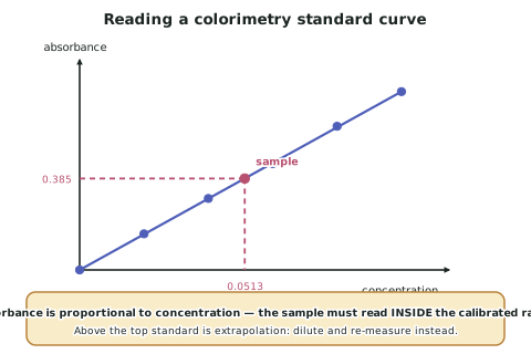
The sample sits inside the calibrated range, so reading across to the line is an interpolation — supported by standards on both sides. Concentration = 0.0513 mol L⁻¹.
Making the curve valid
Explanatory Note 6 requires the range of the standard curve to be appropriate, and this is where colorimetry investigations most often fail.
-
Your samples' absorbances must fall inside the range covered by your standards.
- A sample reading above the highest standard is being extrapolated, not interpolated — and extrapolation beyond the measured range is not supported by the data.
- A sample reading near zero is in the region where the percentage uncertainty is largest.
-
Use at least five standards, spread evenly across the range.
-
Include the origin as a point only if a blank of zero concentration genuinely reads zero absorbance — which it should, if the blank was prepared correctly.
-
If a sample reads off the top of the curve, dilute it by a known factor and re-measure, then multiply back. This is a modification you can justify.
Where the Beer–Lambert law breaks down
-
The linear relationship fails at high concentrations, typically above about . The curve bends towards the concentration axis, so a sample in that region reads lower than its true concentration.
-
Causes include interactions between the absorbing particles at high concentration, and stray light in the instrument.
-
This is why the range matters. A calibration built entirely within the linear region, with samples inside it, is valid; one extending into the curved region is not.
-
Other things to control: the same cuvette, the same orientation, clean and dry outer faces, no bubbles, and consistent temperature.
Colour development reactions
- Some analytes are colourless and must be converted to a coloured species first.
- Fe3+ with thiocyanate gives a deep red complex.
- Phosphate with molybdate and a reducing agent gives molybdenum blue.
- If you use a colour development reaction, the same amount of reagent must be added to every standard and every sample, and the same development time allowed — otherwise the colour intensity varies for reasons unrelated to the analyte.
Worked ExampleUsing a standard curve
A student measures copper(II) concentration by colorimetry at 620 nm. Standards give the following absorbances:
| [Cu2+] / mol L−1 | Absorbance |
|---|---|
| 0.000 | 0.000 |
| 0.020 | 0.152 |
| 0.040 | 0.301 |
| 0.060 | 0.448 |
| 0.080 | 0.605 |
| 0.100 | 0.751 |
A sample gives an absorbance of 0.385. Determine its concentration, and evaluate whether the reading is reliable.
Step 1 — Check the data is linear
Plotting absorbance against concentration gives a straight line passing through the origin, as the Beer–Lambert law predicts. Checking the ratio at each point:
The ratios agree to within about 1%, confirming the relationship is linear across the whole range and that no point lies in the region where the law breaks down.
Step 2 — Find the gradient of the line of best fit
Using the extreme points on the line of best fit:
So the calibration is:
Step 3 — Read off the unknown
Step 4 — Check the reading is an interpolation
The sample's absorbance of 0.385 lies between the standards at 0.301 and 0.448, so its concentration is being read inside the calibrated range — an interpolation, which the data supports.
Had the absorbance been above 0.751, the value would have been an extrapolation beyond the measured range, unsupported by the data and additionally suspect because the Beer–Lambert law tends to fail at higher absorbances.
Step 5 — Significant figures
The absorbances were recorded to 3 decimal places and the standard concentrations to 2 significant figures... in fact 0.020 to 0.100 mol L−1 carry 2–3 sf. Taking the standards as 3 sf and the absorbance reading as 3 sf, the answer is quoted to 3 significant figures.
Step 6 — Evaluate the reliability
- The linearity check across five standards is strong evidence that the calibration is valid over this range.
- The sample sits near the middle of the range, where the relative uncertainty in reading off the line is smallest.
- Residual concerns: the same cuvette must have been used throughout in the same orientation, since small differences in glass thickness or scratches change the path length ; and the blank must have contained every reagent except the copper, or the intercept would not be zero.
Answer: the sample contains Cu2+ at 0.0513 mol L−1, read by interpolation from a calibration that is linear across the full range measured.