Fitting a model, predicting, and the conclusion
Choosing the model
- Look at the scatter plot and match the model to the shape. This is the decision, and it comes before any fitting.
- Points scattered about a straight line → linear model
- Points following a curve → non-linear model
- The standard explicitly permits non-linear relationships. Forcing a straight line onto curved data is a substantive error, not a simplification.
The linear model
-
is the slope — the change in for a one-unit increase in .
-
is the intercept — the predicted when .
-
Interpreting the slope is where the marks are, and it must be done with both variables' units and the context:
- Not: "the slope is "
- But: "the slope is , meaning that for each additional 1 000 km on the odometer, the predicted sale price falls by about $43."
-
Interpreting the intercept requires care. It is only meaningful if is within or near the data range and makes sense in context. If your data covers houses of 80–300 m2, the intercept describes a house of zero floor area, which is meaningless — say so rather than interpreting it.
Residuals
- A residual is the vertical distance from a point to the fitted model:
- A positive residual means the actual value is above the model; negative means below.
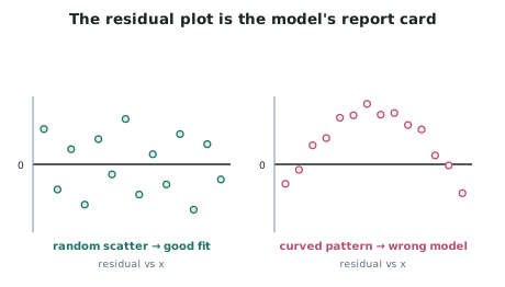
- The residual plot is the model's report card. Plot residuals against and look:
| What the residual plot shows | What it means |
|---|---|
| Random scatter about zero | The model fits the shape of the data |
| A curved pattern | The relationship is non-linear — wrong model |
| A fan shape | Scatter changes across the range; predictions are less reliable at one end |
| An isolated extreme point | An outlier worth investigating |
- Producing and interpreting a residual plot is one of the clearest ways to evidence "evaluating the adequacy of the model", which is named in the Excellence criterion.
Making a prediction
- Substitute your value into the model and state the result in context, with units.
- Then qualify it. Three things must be said:
- The uncertainty. "Given the scatter, actual prices for a car with this odometer reading have ranged from about $8 000 to $16 000, so the prediction of $12 000 should be read as a central estimate rather than an exact figure."
- Whether it is interpolation or extrapolation.
- Whether the scatter is larger at that part of the range.
Interpolation and extrapolation
- Interpolation — predicting within the range of the data. Reasonable.
- Extrapolation — predicting outside it. Unreliable, and often nonsensical.
- Say which you are doing, every time. Extrapolation fails because there is no evidence the pattern continues beyond the data, and a linear model extended far enough will eventually predict impossible values — negative prices, negative times, percentages above 100.
Association is not causation
- A fitted model shows that two variables move together. It does not show that one causes the other.
- Three alternatives always exist, and naming the relevant one is a contextual judgement:
- A confounding variable influences both.
- The causation runs the other way.
- Chance, particularly in a small data set.
- Say this explicitly in the conclusion, and name the specific alternative that applies to your context — not the generic phrase.
The conclusion
- A conclusion that scores well:
- Answers the relationship question posed at the start
- Describes the nature and strength with evidence from the data
- Explains the relationship in context
- States the prediction with its uncertainty and limitations
- Evaluates the model — residuals, whether the form was right, where it is least reliable
- Considers other relevant variables and says what each would add
- Notes limitations — the data set's origin, its size, whether the population is narrow
Worked ExampleFitting, predicting and concluding
A student investigating house floor area (m2) against sale price ($000s) for 120 sales in one New Zealand suburb has fitted:
The data cover floor areas from 75 m2 to 240 m2. At a floor area of 150 m2, observed prices in the data range from about $620 000 to $920 000. The residual plot shows random scatter but with the spread widening as floor area increases.
Write the model interpretation, a prediction for a 160 m2 house, and the conclusion.
Step 1 — Interpret the slope
Step 2 — Interpret the intercept, carefully
Step 3 — Make the prediction
For a floor area of 160 m2: