Error bars and the uncertainty in a gradient
Why the graph has to show the uncertainty
At Level 3 the graph must carry the uncertainty, not just the values. That is what the criteria mean by "graphical analysis including a consideration of uncertainties".
- An error bar is a line drawn through a plotted point extending one uncertainty above and one below it, with a small cap at each end.
- Draw error bars on the axis whose uncertainty is significant — usually the vertical axis. If the horizontal uncertainty is negligible in comparison (say, less than a fifth of the vertical one), say so and leave it off.
- The uncertainties plotted must be the propagated ones for the linearised quantity, not the raw ones.
- If you plot and has a uncertainty, the error bar on is — the power rule.
Getting an uncertainty on the gradient
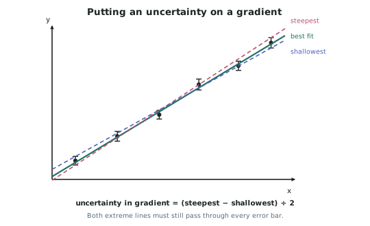
- Draw the line of best fit through the points.
- Draw the steepest line that still passes through every error bar.
- Draw the shallowest line that still passes through every error bar.
- Find the gradient of each extreme line, and take half the difference:
- Quote the result as , with the uncertainty to one significant figure.
Both lines pass through every error bar, so the gradient is 1.84 ± 0.10. Widen them and the uncertainty grows for no reason — quote the tightest pair that still works.
- Drag each line and watch which points turn red. A line only counts as an extreme if it passes through every error bar — one miss and it is not usable.
- Push the lines wider than they need to be and the uncertainty grows for no reason. The correct answer is the tightest pair that still work, because a needlessly large uncertainty makes the comparison with theory meaningless.
Rules that markers look for
- Both extreme lines must pass through all the error bars, not most of them.
- Both extreme lines should be plausible fits — usually pivoted about the middle of the data rather than hinged at one end.
- Gradients must be read from points on the lines, taken far apart.
- The gradient uncertainty must be consistent with the scatter in the data: if the points are tightly grouped, a huge quoted uncertainty is as wrong as a tiny one.
Turning a gradient uncertainty into a quantity uncertainty
- If a physics quantity is calculated from the gradient, the percentage uncertainty carries through by the ordinary rules.
- Gradient s2 m−1 has .
- For a pendulum, , so inherits the same (dividing by a quantity passes its percentage uncertainty straight through; is exact).
- m s−2, and of is , so m s−2.
Worked ExampleFrom error bars to a value of g with its uncertainty
A pendulum investigation gives a graph of against with error bars. The line of best fit has gradient s2 m−2, the steepest acceptable line has gradient and the shallowest . Find the gradient with its uncertainty, and use to find with its uncertainty.
Step 1 — Find the uncertainty in the gradient
So the gradient is s2 m−1.
Step 2 — Express it as a percentage uncertainty
Step 3 — Relate the gradient to
Squaring the theory, , so the gradient of against is , giving
Step 4 — Carry the percentage uncertainty into
is an exact number, so it contributes no uncertainty. Dividing by passes 's percentage uncertainty straight through:
Step 5 — Compare with the accepted value
The accepted value m s−2 lies comfortably within to m s−2, so the data supports the theory.