Optimising: the corner-point and sliding-line methods
The corner-point method
- The theorem: a linear objective attains its optimum at a corner of the feasible region.
- The method, in four steps:
- Find every corner exactly, by solving pairs of boundary equations.
- Evaluate the objective function at each corner, showing the substitution.
- Select the largest value (for a maximum) or the smallest (for a minimum).
- State the answer in context, with the decision and the objective value.
- Set the evaluation out as a table. It makes the comparison checkable and it is what assessors look for:
| Corner | Value | |
|---|---|---|
| $300 | ||
| $2,400 | ||
| $2,600 | ||
| $2,200 | ||
| $1,900 |
- Show the arithmetic, not just the totals. A single mis-multiplied corner changes the answer, and visible working lets it be found.
The sliding-line method
- The alternative, and the one that explains why the corner method works.
- The objective defines a family of parallel lines, one for each value of :
- Every line in the family has the same gradient, here . Only the intercept changes.
- The method:
- Draw one line of the family — pick a convenient , such as , giving intercepts and .
- Slide it parallel across the region, in the direction that increases .
- The last corner it touches before leaving the region is the optimum.
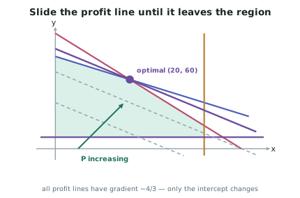
- Which way does increase? For an objective with positive coefficients, increases away from the origin. Test two lines if unsure — evaluate at two points and see which is larger.
- Use a ruler and keep the gradient exact. A slightly wrong gradient picks the wrong corner, and the error is invisible in the final number.
Which method to use
| Situation | Better method |
|---|---|
| Few corners, exact values needed | Corner-point — it is exact and shows working |
| Many corners | Sliding line — it finds the optimum without evaluating all of them |
| Explaining why the answer is optimal | Sliding line — the geometry is the explanation |
| Detecting multiple optima | Sliding line — a tie is visible as an edge, not a point |
- Do both when time allows. The corner-point method gives the number; the sliding line confirms it and shows the reasoning. Agreement between them is a strong check.
Multiple optimal solutions
- When the objective line is PARALLEL to a binding edge, every point on that edge is optimal.
- Detect it by comparing gradients: the objective has gradient ; a constraint has gradient . Equal gradients mean a possible tie.
- It shows up in the corner table as two corners with the same value.
- Report the whole edge, not just one end: "any plan on the line from to gives the same profit". In context this is good news — the business gets to choose on other grounds.
Minimisation problems
- The method is identical; only the selection changes — take the smallest corner value.
- Minimisation contexts are usually about cost: feed mixes, transport, staffing.
- The constraints are usually ("must supply at least"), so the region is often unbounded above — which is fine, because the minimum still sits at a corner on the lower boundary.
Reporting the answer
- State the decision, the objective value and the binding constraints:
- "Make 20 trays of Halloumi and 60 of Feta, for a weekly profit of $2,600."
- "Both the vat and the packing line are fully used; cold storage has 20 trays of spare capacity."
- Say what the business should do with that information. The binding constraints are the ones worth expanding.
Worked ExampleOptimising the dairy model
Using the feasible region already found — corners , , , and — maximise for the dairy, confirm the answer with the sliding-line method, and advise the company.
Step 1 — Evaluate the objective at every corner
Corner :
Corner :
Corner :
Corner :
Corner :
Step 2 — Select the maximum
| Corner | Profit |
|---|---|
| $300 | |
| $2,400 | |
| $2,600 | |
| $2,200 | |
| $1,900 |
Note that the highest- corners are NOT best, even though Halloumi is the more profitable product per tray. It uses twice the vat time, so the extra $10 of profit does not pay for the extra hour.
Step 3 — Confirm with the sliding-line method
Write the objective as a line family:
Every profit line has gradient .
Draw a trial line, say : intercepts and .
Slide it away from the origin, since both coefficients are positive and therefore increases in that direction.
Compare the gradients of the boundary edges:
| Edge | Constraint | Gradient |
|---|---|---|
| Vat | ||
| Packing | ||
| Objective |
The objective's gradient, , lies BETWEEN the vat edge () and the packing edge ().
The two methods agree ✓
Step 4 — Identify the binding constraints
At :
| Constraint | Value | Status |
|---|---|---|
| Vat: | BINDING — all 100 hours used | |
| Packing: | BINDING — all 80 hours used | |
| Storage: | slack — 20 trays spare | |
| Contract: | slack — 50 trays above the minimum |
Step 5 — Report to the company
Step 6 — Advise on what to expand
Since storage and the contract are slack, expanding either buys nothing. The two constraints worth relaxing are the vat and the packing line.
Test one extra vat hour — the constraint becomes , so the corner moves to where meets :
Gain: $10 per extra vat hour.
Test one extra packing hour — with :
Gain: $20 per extra packing hour.
A caution on that advice. These marginal values hold only while the same two constraints stay binding. Add enough packing hours and the storage limit or the vat limit eventually takes over, at which point the extra hours stop being worth $20 — so the advice is "buy some", not "buy unlimited".