The manipulations
The closed list, and what Level 3 does with it
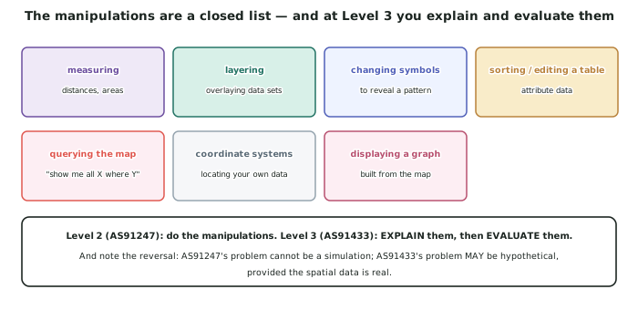
- The standard names seven manipulations and the list is closed: measuring, layering, changing symbols, sorting and editing a table, querying the map, using coordinate systems, and displaying a graph based on the map.
- At Level 2 (AS91247) the manipulations only have to be done. At Level 3 they must be EXPLAINED, and at Excellence EVALUATED.
- Explaining a manipulation means saying what it did, why it was the right tool, and what its output means.
- Evaluating a manipulation means judging how well it worked — its assumptions, its error, and what a different technique would have produced.
- Use several. A project using one manipulation has not really done spatial analysis, and most real problems need four or five.
Layering, which is usually the core of the analysis
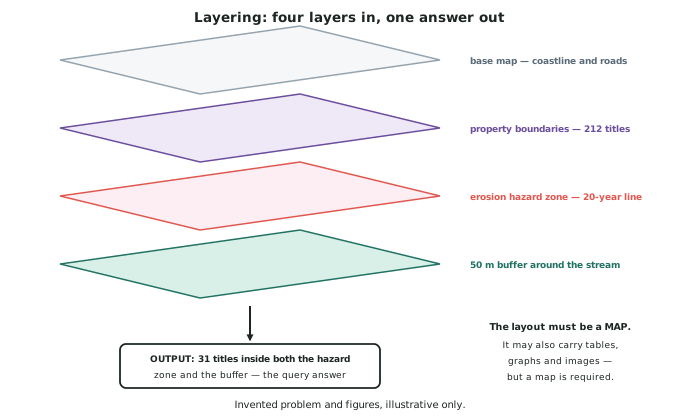
- Layering means overlaying datasets so that conditions can be combined. It is what makes GIS more than a drawing program.
- Order matters for clarity, not for the result: put the base map at the bottom, polygons above it, lines above those, points on top.
- The analytical operation is usually an intersect — keep only what is inside every layer — or an erase, which removes what is inside a constraint.
- Apply hard constraints first. Remove the hazard zone and the flood extent before testing distance criteria, because it is faster and the intermediate maps are easier to read.
- In the invented Ōtaraki problem, four layers combine: the base map, the property parcels, the 50-year hazard zone, and a 50 m stream buffer — and the output is the land that is inside none of the constraints.
Buffering, measuring and querying
- A buffer is a measured zone around a feature — the 50 m riparian setback, or the 1 km service catchment. It is measuring and layering used together.
- Say where the buffer distance came from. A number pulled from nowhere is an assumption; a number from a district plan is a criterion.
- Measuring covers distances and areas, and it is where coordinate systems matter most: an area calculated in an unprojected coordinate system is wrong.
- Querying the map is show me all X where Y — the manipulation that turns a picture into an answer. In the invented problem: select all parcels where area ≥ 0.4 ha AND outside hazard AND outside buffer AND within 1 km of services.
- Record your query in full, in the report. It is the most checkable evidence of what you actually did, and it is worth more than a screenshot.
Symbols, tables and graphs
- Changing symbols is a manipulation, not decoration, when it is used to reveal a pattern: graduated colours by a value, proportional symbols by size, or a two-class shading of pass and fail.
- Sorting and editing a table is how you work with attributes — sort parcels by area to see how many clear the minimum, or add a field recording which criterion each parcel failed.
- Adding a "reason failed" field is one of the most useful edits you can make, because it converts a yes/no map into a diagnosis and it tells you which criterion is doing the work.
- Displaying a graph based on the map links the two: a bar chart of how many parcels each criterion eliminated shows which condition is binding.
- Every one of these is on the standard's list, so using them and explaining them is directly creditable.
Explaining a manipulation properly
- Four moves: what you did, why that tool, what the output is, and what it means for the problem.
- Worked example: I applied a 50 m buffer to the stream centrelines (what), because the district plan measures its riparian setback from the centreline and a buffer reproduces that rule exactly rather than approximating it (why). The output is a polygon of 14.2 ha covering the restricted land (output), which removed 3 of the 27 candidate parcels from consideration (meaning).
- Quantify the effect of every manipulation. It removed 3 of 27 parcels is what turns a description of software use into analysis.
- Include the manipulations that changed nothing, and say so — a criterion that eliminates no parcels is telling you something about the site.
- Screenshots support the explanation; they do not replace it.
Worked Example
Worked example
Explain the manipulations used to solve the invented Ōtaraki relocation problem.
Answer:
Manipulation 1 — using coordinate systems.
What: all five layers reprojected to NZTM2000. Why: three of my five criteria involve distances or areas, and both are wrong if calculated across mismatched coordinate systems. Output: a project in which every layer aligns. Meaning: without this step the buffer, the service distance and the parcel areas would all have been silently incorrect — the map would have looked identical and the answer would have been wrong.
Manipulation 2 — layering, with an erase.
What: the 50-year hazard zone and the flood extent erased from the candidate area. Why: these are hard constraints — land inside them cannot be used, so removing it first reduces everything that follows. Output: a candidate area reduced from 312 ha to 196 ha. Meaning: the hazard constraint alone removed 37 per cent of the study area, which is the first indication that suitable land is genuinely scarce here.
Manipulation 3 — buffering, which is measuring plus layering.
What: a 50 m buffer applied to the stream centrelines and erased from the candidate area. Why: the district plan measures its riparian setback from the centreline, so a buffer reproduces the rule exactly. Output: a 14.2 ha restricted polygon. Meaning: it removed 3 of the 27 parcels still in contention, all in the eastern gully.
Manipulation 4 — sorting and editing the attribute table.
What: parcels sorted by area, and a new field added recording which criterion each failing parcel failed. Why: a yes/no output cannot tell you which condition is binding, and that is what the justification needs. Output: a table showing that 11 parcels qualify and that of the 16 that fail, 9 fail on the hazard criterion, 3 on the buffer and 4 on lot size. Meaning: hazard is the binding constraint, not lot size — which is not what I expected.
Manipulation 5 — querying the map.
What: the full query — select parcels where area ≥ 0.4 ha AND NOT within hazard_50yr AND NOT within stream_buffer_50m AND NOT within flood_extent AND within 1 km of service_network. Why: it applies all five criteria at once and produces the answer as a selection rather than as a visual judgement. Output: 11 parcels, totalling 6.8 ha. Meaning: enough land for the 14 properties only if some sites are subdivided to the minimum lot size.
Manipulation 6 — displaying a graph based on the map.
What: a bar chart of how many parcels each criterion eliminated. Why: it makes the binding constraint visible at a glance. Output: hazard 9, lot size 4, buffer 3, services 0. Meaning: the service-distance criterion eliminated nothing, so it is not doing any work here — a result worth reporting, because it means relaxing it would not help.